Exploratory data analysis and visualisation using QGIS

In this exercise

• How to use QGIS (http://qgis.org) as a tool for interacting with data using web data services and on the VDI filesystem
• Obtaining data from a Web Coverage Service (WCS)
• Obtaining data from a web-based vector data service
• Obtaining data from the NCI file system using the NetCDF Operators (NCO)
• Using QGIS to fuse data and create a shareable, interactive 3D map rendered using webGL in a browser

We are going to make an interactive version of the map below, starting with data from three different sources merged using QGIS. We will also see some key differences between data access methods.

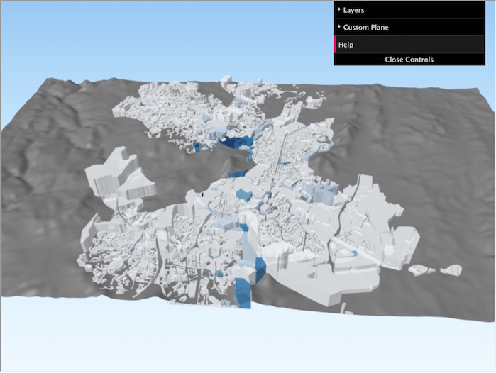
The following material uses Geoscience Australia’s Elevation Data Collection which is available under the Create Commons License 4.0 through NCI’s THREDDS Data Server. For more information on the collection and licensing, please click here. Also used is ANU Water and Landscape Dynamics tree cover product, available under the Create Commons License 4.0 through NCI’s THREDDS Data Server. For more information on the collection and licensing, please click here

What is QGIS?

QGIS (Quantum GIS) is an application for geospatial data analysis and visualisation, focussed on 2D (raster and vector) datasets, and wrapped in a straightforward graphical user interface. It can also be used as a Python library, but for this session we use the GUI.

I have [insert many other tools] on the VDI - why use QGIS?

QGIS can be used on the VDI as a rapid-prototyping tool. If you’ve got all the infrastructure you need available in your project space and don’t need it, that’s great! We hope to demonstrate some ways which QGIS can help you quickly develop shareable, multi-source analyses quickly and simply. We also revise some web service principles.

1. Define a question and create some spaces

For this session the question we want to address is:

• How are the ‘hilliness’ of suburban areas and and ‘tree cover’ in Canberra related?; and
• do hillier sections have more or less tree cover than flatter sections?

Before we forge ahead, let’s make a project space - in the terminal head to your home directory and create something like:

$ mkdir ./qgis_vis_files

…to hold some data subsets we will create, and:

$ mkdir ./qgis_vis_map

…to hold our finished map. We will use these throughout the session.

2. Decide on some useful datasets

To answer our question we need some data on topography, vegetation and where block boundaries are. From NCI’s collections we can use:

• A Shuttle Radar Topography Mission raster DEM at 1 arc-second resolution: /g/data/rr1/
• Some tree cover indices from the ANU Water and Landscape Dynamics collection: /g/data2/ub8/

NCI doesn’t hold cadastral data, so we’ll get those from the local land administrator:

• ACT cadastral data outlining sections (held outside NCI)

Note - here, sections are collections of 50 or so individual house blocks. Our elevation and tree cover data are too coarse for individual house blocks - and the vector data file for blocks is massive!

3. Take a look at the data held at NCI

Elevation

We use an SRTM elevation mosaic, held in Geoscience Australia’s elevation reference collection:

THREDDS

http://dapds00.nci.org.au/thredds/catalog/rr1/Elevation/NetCDF/catalog.html

Geonetwork

https://geonetwork.nci.org.au/geonetwork/srv/eng/catalog.search#/metadata/f9082_1236_9859_8989

Licensed under Creative Commons (CCBY4): http://dapds00.nci.org.au/thredds/fileServer/licenses/rr1_licence.pdf

The path to the data on your VDI desktop is:

/g/data1/rr1/Elevation/NetCDF/

As a demonstration, we will acquire these data using a Web Coverage Service (WCS).

Tree cover

We will extract tree cover data from the filesystem. These data come from the ANU Water and Landscape Dynamics collection:

THREDDS

http://dapds00.nci.org.au/thredds/catalog/rr1/Elevation/NetCDF/catalog.html

Geonetwork

http://geonetwork.nci.org.au/geonetwork/srv/eng/catalog.search#/metadata/f1104_2906_7276_3004

The path to the data on your VDI desktop is:

/g/data1/ub8/Elevation/NetCDF/

4. Start QGIS on the VDI

Like most VDI applications, we use the module load system to acquire QGIS, GDAL and NCO:

module purge
module load gdal-python/1.11.1-py2.7 qgis/2.14.8-py2.7
qgis &

This will start QGIS - which we’ll use shortly. For now, head to Firefox - we are off to discover some data! Note - we’ve also loaded NCO, which we will get to soon.

5. Get topography data using Web Coverage Services

For topography we need a terrain model in a raster format, e.g. GeoTIFF, which covers Canberra. Shuttle Radar Topography Mission (SRTM) data are a good source of reasonably detailed elevation data held at NCI as NetCDF tiles.

We can head to the NCI Elevation collection here:

http://dapds00.nci.org.au/thredds/catalog/rr1/Elevation/catalog.html

…and look for SRTM 1 second elevation as NetCDF. Browse to the NetCDF folder, click through to:

http://dapds00.nci.org.au/thredds/catalog/rr1/Elevation/NetCDF/1secSRTM\_DEMs\_v1.0/DEM/catalog.html

A bunch of 1 degree tiles are shown here - but we will collect a region we want from the national mosaic:

http://dapds00.nci.org.au/thredds/catalog/rr1/Elevation/NetCDF/1secSRTM\_DEMs\_v1.0/DEM/catalog.html?dataset=rr1/Elevation/NetCDF/1secSRTM\_DEMs\_v1.0/DEM/Elevation\_1secSRTM\_DEMs\_v1.0\_DEM\_Mosaic\_dem1sv1\_0.nc

Click on the ‘WCS’ link to see the WCS getCapabilities statement - which describes the data you can obtain here. We need to know the name for the coverage we need - look for the ‘name’ tag. With that,and using our WCS knowledge, we can request just the part of the data we need and acquire a GeoTIFF image. Let’s break a WCS request down into parts we need:

• the path to the data: http://dapds00.nci.org.au/thredds/wcs/rr1/Elevation/NetCDF/1secSRTM_DEMs_v1.0/DEM/
• the dataset: Elevation_1secSRTM_DEMs_v1.0_DEM_Mosaic_dem1sv1_0.nc
• the service: service=WCS
• the service version: version=1.0.0
• the thing we want to do (get a coverage): request=GetCoverage
• the coverage (or layer) we want to get: Coverage=elevation
• the boundary of the layer we want: bbox=148.7,-35.8,149.5,-35.1
• the format we want to get our coverage as: format=GeoTIFF_Float

To build a WCS request we concatenate the data path and dataset name, put a question mark after the dataset name, then add the rest of the labels describing the thing we want afterward, in any order, separated by ampersands:

Enter this link into a web browser to obtain a GeoTIFF DEM in your default download location (check in ‘downloads’). Rename it to something memorable if you wish, in your qgis_vis_files directory.

Note the use of GeoTIFF_Float - using only GeoTIFF is possible, but gives you an image with pixel values scaled to a colour range, not a data range

Now go to QGIS and import the GeoTIFF as a raster layer:

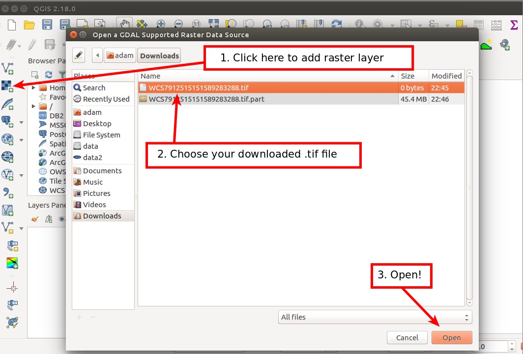
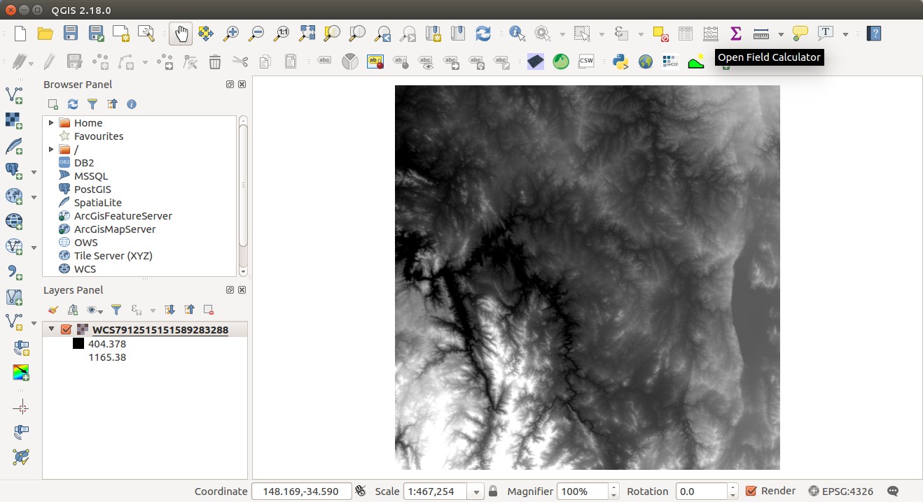
6. Acquire tree cover data from the file system

Here we pull some data from a netCDF file straight from the NCI file system - but we don’t want all of Australia - let’s stick to our region of interest, and use NCO to grab the part we need. In a new terminal move to your qgis_vis_files directory and load the NetCDF Operators:

$ module load nco/4.5.3

…which we use to clip a region from the ANU WALD TreeCover dataset for 2015:

$ ncks -v TreeCover -d latitude,-35.8,-35.1 -d longitude,148.7,149.5  /g/data1/ub8/au/treecover/ANUWALD.TreeCover.25m.2015.nc ./treecover_2015_-35.8-35.1_148.7_149.5.nc

QGIS will panic if you attempt to load your new netCDF subset, because it misinterprets the order of latitude and longitude. A quick call to another NCO utility fixes that - here we swap the axis order in the TreeCover variable for our subset:

$ ncpdq -v TreeCover -a latitude,longitude treecover_2015_-35.8-35.1_148.7_149.5.nc treecover_2015_-35.8-35.1_148.7_149.5.nc

This results in a subset of the ANU WALD treecover dataset in our VDI desktop - which we can load into QGIS as a raster layer.

You could just as easily load a complete NetCDF file from /g/data into QGIS - as long as the underlying file format meets defined netCDF conventions. Try adding this gravity map - it meets NetCDF-CF, and loads without any modification: /g/data/rr2/National_Coverages/onshore_Bouguer_offshore_Freeair_gravity_geodetic_June_2009/ onshore_Bouguer_offshore_Freeair_gravity_geodetic_June_2009.nc

Here, we demonstrate a method of quickly viewing parts of your output data - even if they are not yet fully QC'ed and need a little massaging to get going.

7. Style our tree cover layer

So far we have a bunch of grey things - let’s make them colourful!

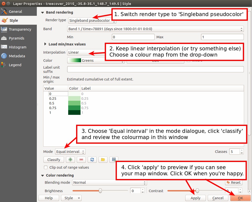
We don’t need to worry about the elevation data, but we do need a useful colour scheme for vegetation data and our cadastral data. Double click your vegetation layer (in the layers panel) to bring up it’s properties dialogue. From there:

• click ‘style’
• in the ‘render type’ dropdown, choose ‘Singleband pseudocolor’
• leave interpolation as ‘linear’, and pick a colour palette. Because the data are continuous, a single hue continuous colour palette makes sense. Because it’s vegetation, green also makes sense. Choose what makes sense to you.
• click ‘classify’ to show the palette in the big window, and apply with with ‘apply’.
• click ‘close’ to return to your map.

Extension:

Steaming ahead? Add a graticule to your QGIS map layer...

How could you automagically save WCS data with sane, memorable names?

Q & A

Why not just use the QGIS OWS browser to grab these data?

1. The QGIS WCS browser and THREDDS don't play well - QGIS attenuates the full THREDDS WCS URL, so it is far more convenient to form a request independently of QGIS.
2. OWS layers can't be used for processing - ie band math, and the visualisation tools we're about to use.

If you're keen, do some exploring - we don't know everything about QGIS - surprise us!

Why not get these data from the filesystem?

Great question! The main reason is that we're demonstrating QGIS as a way to fuse data from manifold sources. Over today and tomorrow you'll see a log examples of how to collect data from the filesystem in manageable chunks - which you could then analyse/visualise using the methods shown here. Demonstrating web coverage services on the VDI shows how you can pull data from many external sources to help interpret your work.

8. Find a cadastral data service and import it into QGIS

Finding and importing data as a service

ACT publish a lot of spatial data on their ACTMAPi interface. To shortcut, here are the cadastral section data:

http://actmapi.actgov.opendata.arcgis.com/datasets/eedcda7873934e789093b093521b0299\_3

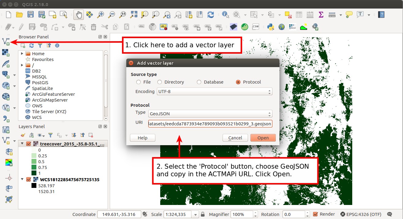
You can download a shapefile and import it to QGIS, but let’s show a feature you might like to use: adding vector data as a service. At ACTMAPi, click the ‘API’ menu box, and copy the URL out of the GeoJSON tetxtbox:

http://actmapi.actgov.opendata.arcgis.com/datasets/eedcda7873934e789093b093521b0299\_3.geojson

In QGIS, Click ‘add new vector layer’, select the ‘protocol’ radio button, and past the URL in.

Making the data useful - reload as a local vector layer

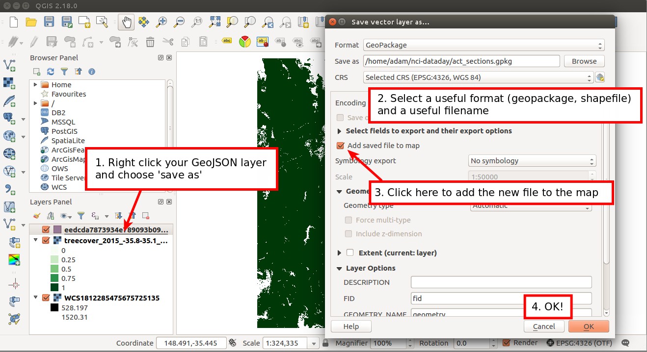
The layer will load - but like WCS raster data, it can’t be used for analysis. Save it as a Geopackage and reload the layer (delete the GeoJSON layer). Again, your qgis_vis_files directory is a good place.

Extension:

Why would we use a Geopackage? Why not a shapefile?
Hint: http://www.geopackage.org

9. Install two useful QGIS plugins

To procees we need to install two QGIS plugins - Qgis2threejs and Zonal statistics :

• Head to the plugins menu and choose manage and install plugins
• In the resulting dialogue box, search for Qgis2threejs
• Select the Qgis2threejs plugin and click install.

The Zonal Statistics plugin is installed by default but needs activating. Search fit Zonal statistics in the plugin manager, and check the box next to the plugin name. Then click close and you’re done.

10. Using zonal statistics for basic analysis

We are aiming to show:

• Standard deviaton of elevation of blocks as a proxy for hilliness; and
• The mean treecoveer of each section.

The Zonal statistics plugin collects data from raster layers using polygons in a vector layer, and computes basic statistics for the chunk of the raster layer inside each polygon.

Section hilliness

As a proxy for section hilliness, we’ll use the standard deviation of elevation in each section polygon. Head to raster -> zonal stats to open the plugin.

In the zonal statistics plugin dialogue, choose the DEM as the raster layer, and use band 1. Then choose your ACT blocks vector layer. In the statistics to calculate, pick an appropriate set - but include standard deviation - this is our roughness proxy. Add a meaningful prefix to the statistics (e.g. ‘dem_’), so you can find them when you need to use them.

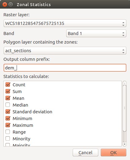
QGIS will spend some time calculating stats for each block, and add the output to the vector layer (act_sections) as another attribute column.

Tree cover per section

For tree cover, each grid cell/pixel shows an estimate of tree cover as a percentage of the pixel. As a quick measure we could take the mean of all the pixel values inside a block to get an idea of it’s tree coverage.

In the zonal statistics plugin dialogue, choose the tree cover as the raster layer, and use band 1. Then choose your ACT sections vector layer. In the statistics to calculate, the values we need are preselected - we’ll use the mean value for each section. Again, use a meaningful prefix (for example, ‘tree_’)

Use mean tree cover per section to style our vector layer

We avoided styling our vector layer earlier, but now it’s time - since we want to visualise the tree cover in each section.

Double click your act_sections layer to open it’s properties dialogue, and head to the style tab. Here, we want to apply a good looking colour scale based on mean tree cover (the data we just generated). Set up as follows:

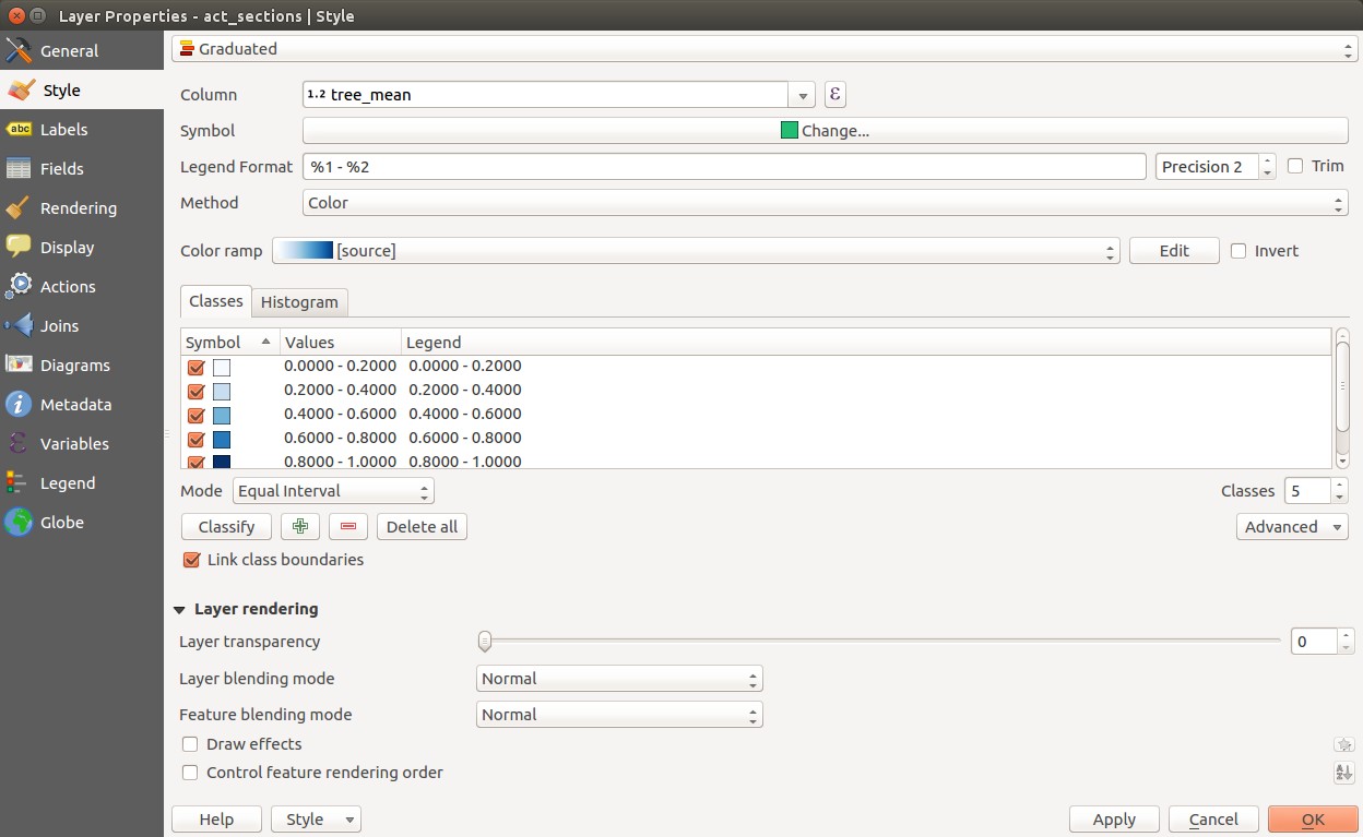
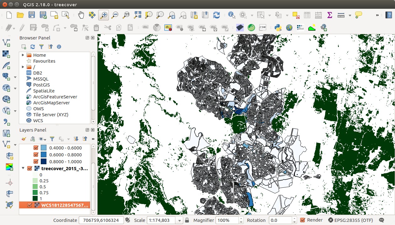
So far we can visualise the tree cover of sections in the ACT - but how can we relate that quickly and easily to section hillines? And how could we visualise results?

is a graphical GIS the only way to collect zonal statistics using a vector layer to segment raster data?

11. Using a simple 3D visualisation to complete the picture

So far we’ve imported three different datasets into QGIS and created some new attributes on our vector dataset. To complete the picture, we will now:

• classify and colour blocks by tree cover
• visualise block hilliness as the height of an extruded column

In this scheme, if hillier blocks have more trees, dark blue blocks will visualise as taller columns. If hiller blocks are less vegetated, light green blocks will visualise as taller columns. Lets test it out!

Here we use the second plugin - Qgis2threejs. This renders the current screen to a WebGL map in a .html page using three.js - with some neat data visualisation features. You can open the result as an interactive map in a web browser.

Setting up - coordinate transformation in QGIS

So far we’ve worked in a WGS84 (EPSG:4326) coordinate system - but in order to render our map in three.js, we need to project our data into something which has units of metres, not degrees. Let’s choose GDA94/MGA55 (EPSG:28355):

• Locate the panel at the lower right of the QGIS window which says ‘EPSG:4326’
• Click it to open a CRS selection dialog
• Select ‘Enable ‘on the fly’ CRS transformation (OTF)’ at the top right
• Enter ‘MGA 55’ in the ‘filter’ box, then highlight GDA94 /MGA 55 in the ‘coordinate systems of the world…’ box. It should show up in the ‘selected CRS’ panel.
• Click OK.

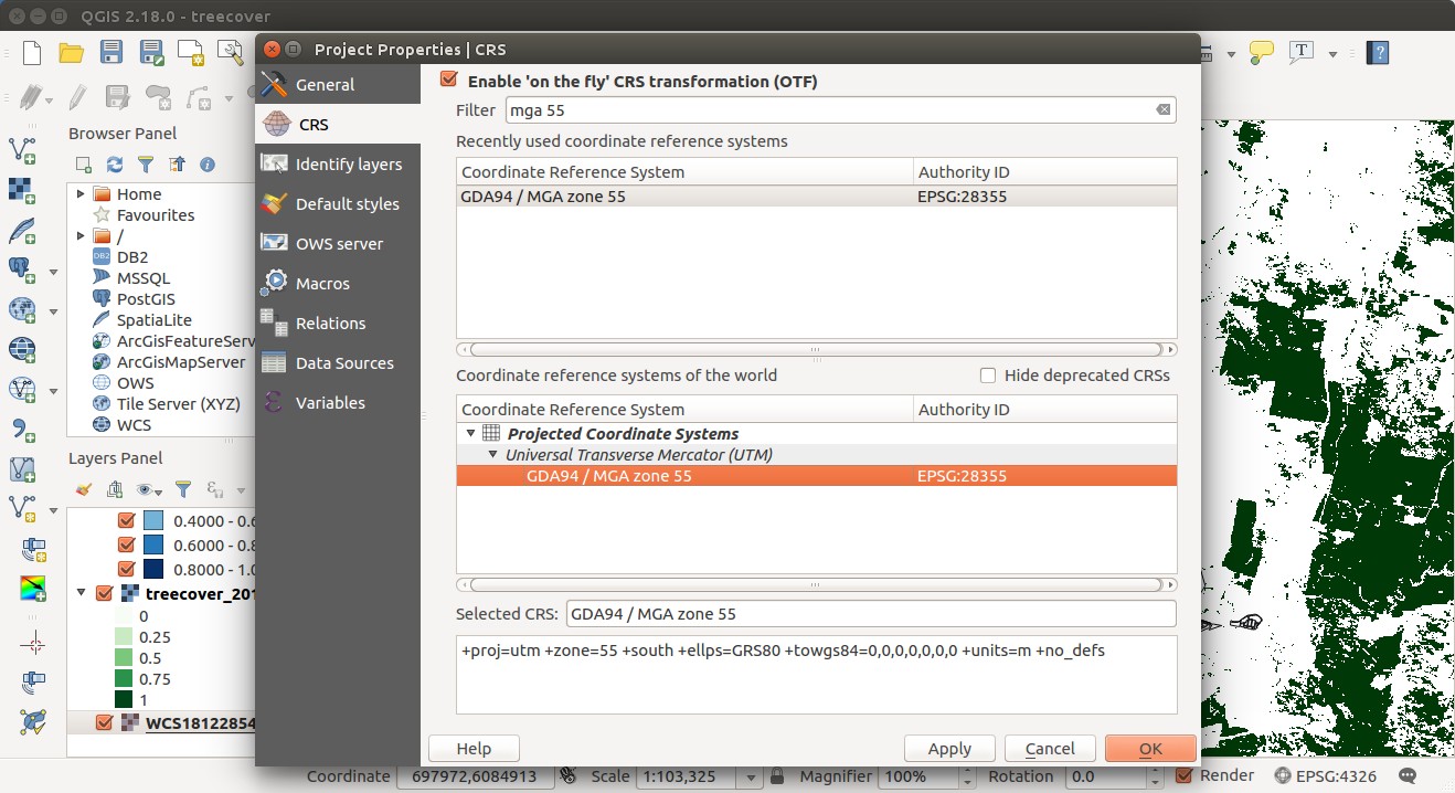
You’ll see that everything has warped a touch, and your CRS panel (lower right) reflects your choice. Proj.4 handles all the rest for you!

Set a clipping frame

Qgis2threejs attempts to render the whole map window. We want to limit or map to the extents of our DEM - so we can either zoom the map window in so that our region of interest occupies the whole window, or set a clipping polygon in a new vector layer. Here, we zoom in so that our region of interest fills the map window.

Setting up in Qgis2threejs

Head to web -> Qgis2threejs to open the plugin dialogue. Click ‘world’ in the left pane, here we define basic parameters about the map we’re creating. It’s usually prettier to apply some vertical exaggeration in Australia, try between 1.5 and 3.

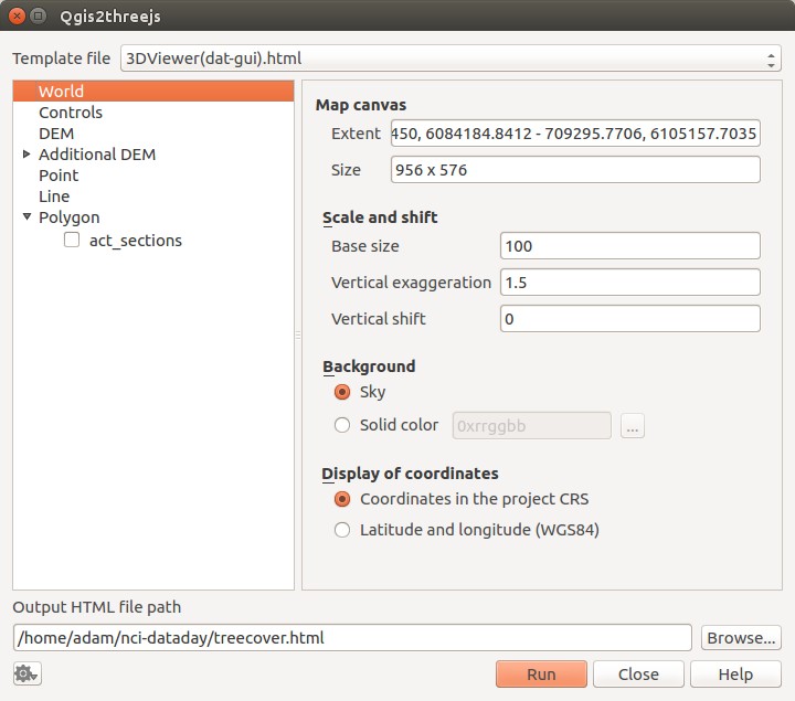
Next click ‘DEM’. Here you select the SRTM data you grabbed via WCS as the dem to build terrain. You can set an image to be draped on the DEM - map window view, a specific layer, an image or a plain colour. This example uses the DEM layer to colour the terrain map. Also turn shading on to get pretty hillshading.

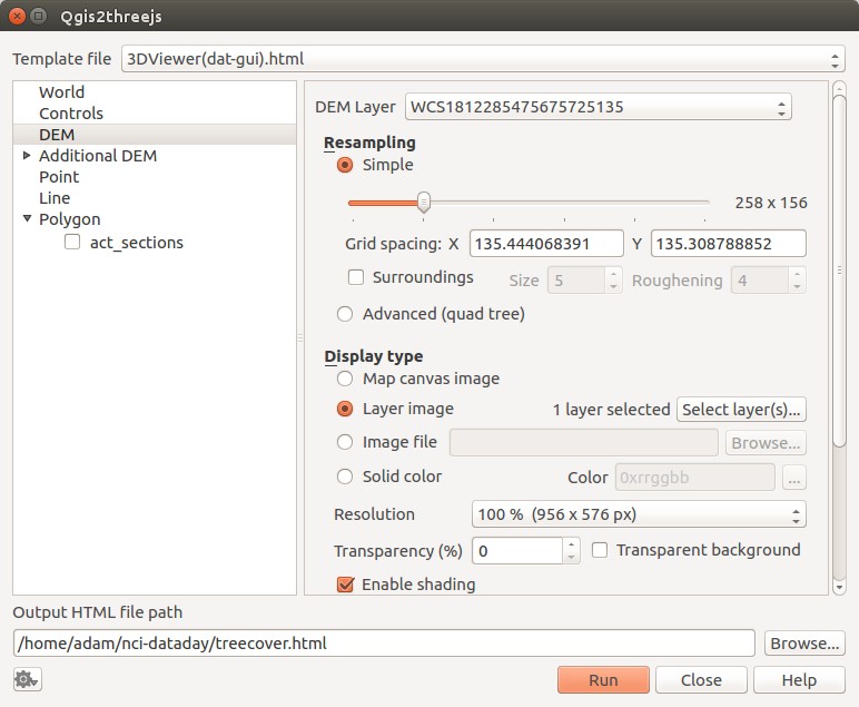
Finally check the radio button next to our ACT sections layer in the left panel. Here we set up some visualisation parameters for our vector layer (which contains the section-level treecover statistics we generated). Set the Z coordinate to’Absolute value’, and enter 580 m. We’re going to compare the heights of extruded polygons, so we should start them all in the same place!

Keep the colour as ‘feature style’, set ‘Transparency’ to 20-30 and finally, choose a data source to detemine extruded polygon heights. We finally relate the hilliness of sections to tree cover here - choose dem_stdev, and a multiplier (10 works well in this example).

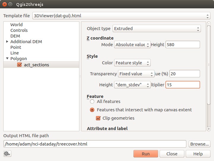
show the map!

We finally use our qgis_vis_map directory - browse to it at the ‘output html file path’ box and use a memorable name to save your output html file. Then click run. All being well firefox will open and display an interactive map like the one below! See section 13 for links to prebuilt versions hosted at github.io.

If the map doesn’t pop up right away navigate to the place you just stored the .html file, and open it in a browser.

12. So what do our results mean? Interpreting our picture

If hilly blocks have generally more tree cover than flatter blocks, short columns should be lighter shades of blue (in this colour scheme).

…but that’s not necesarily what we see! Why not?

Extension activities

• Which suburbs have the most trees? which is the hilliest? hint - use another QGIS plugin, and another web mapping data source - and see the example in section 13
• Create a totally new interactive 3D model using the stack we've just been working with, and give us a URL to see your work!
• Visualise the same result a different way - do we really need qgis2threejs?
<

13. Sharing our new map

The map you just created using QGIS2threeJS can be dropped into any web server - to share with collaborators. You can’t serve data directly from the VDI - but you can copy your qgis_vis_map folder to some web host (e.g. github.io) and share with the world. Here’s an example:

https://adamsteer.github.io/nci\_samples/qgis2threejs/treecover.html

Here’s another example with an OpenStreetMap layer rendered on the DEM:

https://adamsteer.github.io/nci\_samples/qgis2threejs/treecover-osm.html

What are some other ways to share QGIS projects?

Possible solutions to questions

Sane WCS coverage request names

One option is to use curl on the command line:

curl -o SRTM_dem_139_36.tiff 'http://dapds00.nci.org.au/thredds/wcs/ub8/au/FractCov/PV/FractCover.V3_0_1.2015.aust.005.PV.nc?service=WCS&version=1.0.0&Request=GetCoverage&Coverage=PV&bbox=149.0,-36,149.9,-35&format=GeoTIFF_Float'

curl -o 2015_treecover_139_36.tiff 'http://dapds00.nci.org.au/thredds/wcs/ub8/au/FractCov/PV/FractCover.V3_0_1.2015.aust.005.PV.nc?service=WCS&version=1.0.0&Request=GetCoverage&Coverage=PV&bbox=149.0,-36,149.9,-35&format=GeoTIFF_Float'

...are there others? What was yours?

Zonal statistics right in a notebook

You could also try rasterstats: https://github.com/perrygeo/python-rasterstats - any other suggestions?

Other ways to share your QGIS projects, and other 3D visualisers

For simple projects with CCBY4 data, the QGIS cloud is one way of sharing your results. Another is a Jupyter notebook hosted on github as a gist, a notebook, or as a github.io page. What was your approach?

Further reading

Here is a great tutorial on netCDF and QGIS: http://www.ggiuliani.ch/download/netcdf_qgis_GG.pdf - covering a lot more than we did here, and useful for working with data directly on the VDI filesystem.

Also, inspect the result of your work - what is Three.js doing? What can you apply from this example to other work? The Qgis2threejs plugin can only add so much - how could you render additional datasets in the same map? </div> ## Summary Here we: - Used a graphical GIS available on the VDI - Used OGC web services available at NCI - Demonstrated pulling data from external web services - Demonstrated shaping data in the filesystem for merging with web service data - Used these data to perform a basic analysis - Learned one method of visualising and sharing results Thanks! Discussion and suggestions welcome.